Rejection Sampling: The Probability Trick Behind Speculative Decoding

From shaded regions to draft tokens: a visual guide to faster LLM inference with the same output distribution.

In Unpacking Speculative Decoding: The Math Behind the Speedup, we derived the acceptance rate and the expected number of tokens produced in a speculative round. This article takes a closer look at the probability correction that makes the method work.

A small model drafts tokens, and a larger model verifies them together. The challenge is to use those proposals while preserving the larger model’s output distribution.

Why can we keep a small model’s guesses without inheriting its mistakes? Why does the code draw a uniform random number? And why does rejection trigger a subtraction between two distributions?

Let’s start with a picture, then work our way back to the code.

Part 1: Borrow a distribution you can sample from

Suppose we can evaluate a complicated target function, but drawing samples from it directly is inconvenient.

Rejection sampling starts with an easier proposal distribution. It draws candidates from that proposal and filters them so the surviving samples follow the target. Kapil Sachdeva’s visual explanation and companion article provide a helpful introduction. [1]

For the continuous example in this post, define:

$$f(x)=e^{-x^2/2}\left[\sin^2(6+x)+3\cos^2(x)\sin^2(4x)+1\right],\qquad -3\le x\le 3.$$

We restrict this target to −3 ≤ x ≤ 3, and set it to zero outside that interval. This is an illustrative adaptation: every sampler, normalization, and chart below uses that same target.

The function has several peaks. A flat uniform proposal covers the interval evenly; a standard Gaussian concentrates candidates near the middle.

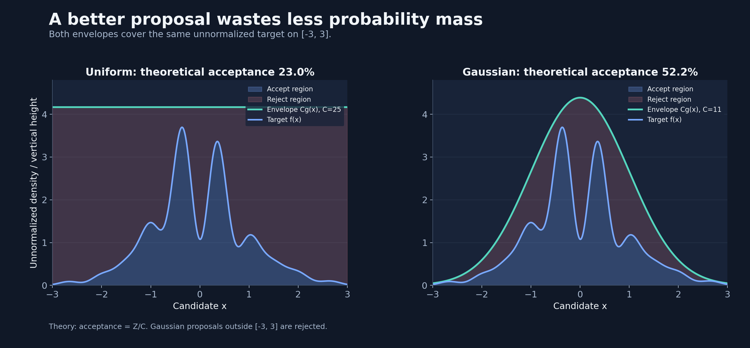
Figure 1. The target is blue; the envelope is teal. Shaded red regions represent rejected draws. For this example, theoretical acceptance rises from 22.95% to 52.16% with the Gaussian proposal.

The proposal itself is a normalized density, g(x). Multiplying by a constant C creates an envelope that must cover the unnormalized target everywhere:

$$C\,g(x)\ge f(x).$$

For our uniform proposal, g(x) = 1/6 on the interval and C = 25. For the Gaussian proposal, g(x) is the standard normal density and C = 11.

An envelope that dips below the target invalidates the sampler. The bound must hold everywhere, not just at the points visible in a plot. Here, the bracketed trigonometric factor is at most 5, so the Gaussian envelope with C = 11 is valid because 11/√(2π) > 5. On the target interval, the uniform envelope has height 25/6; numerical maximization gives a target peak of approximately 3.696.

Part 2: Two random draws have two different jobs

For each proposal, we draw:

1. A candidate x from g(x).
2. A uniform number u from [0, 1).

We accept the candidate if:

$$u < \frac{f(x)}{C\,g(x)}.$$

Equivalently, set a vertical height h = u × C × g(x) and accept when h < f(x). This is the geometric form of the test. [1]

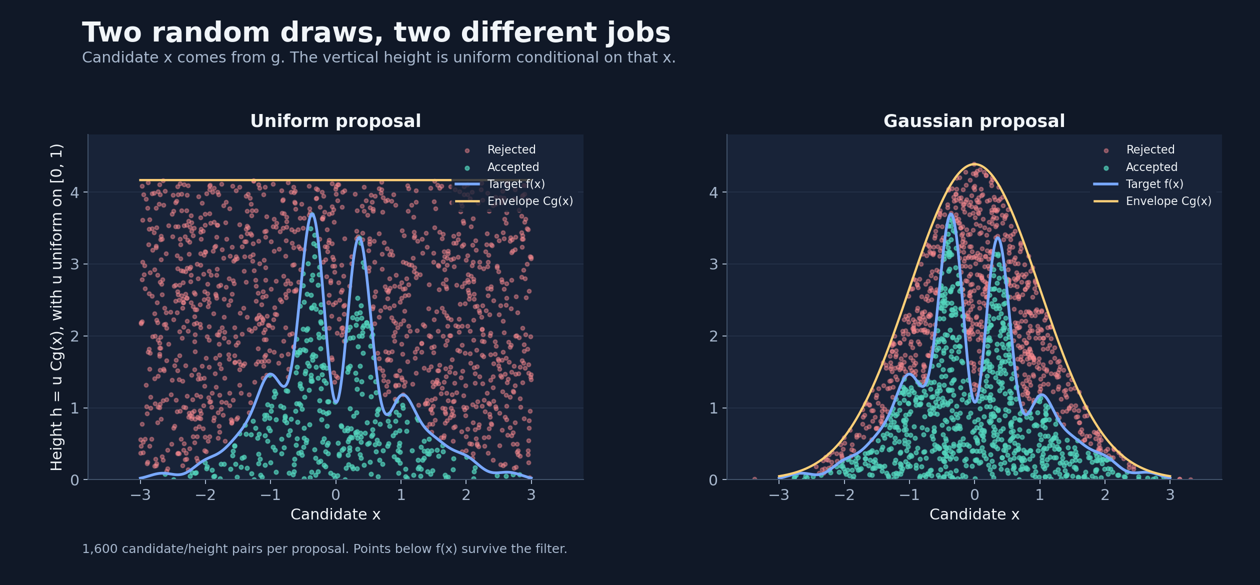
Figure 2. Each dot is one candidate/height pair. A dot below the target survives. The candidate distribution and the conditional uniform height are separate parts of the algorithm.

For a fixed candidate, the acceptance probability is the fraction of its vertical envelope lying below the target curve. That is where the ratio comes from.

The unnormalized density of accepted candidates is therefore:

$$g(x)\frac{f(x)}{C\,g(x)}=\frac{f(x)}{C}.$$

After normalization, the survivors follow f(x)/Z, where Z is the integral of f. We did not need Z to run the acceptance test. We calculate it here to check the results.

Part 3: A better proposal produces the same answers with less waste

For this target, numerical integration gives Z ≈ 5.73807. The expected acceptance rate is Z/C:

Proposal	C	Theoretical acceptance	Observed acceptance
Uniform on [−3, 3]	25	22.95%	22.93%
Standard Gaussian	11	52.16%	52.12%

Each simulation uses 300,000 proposals. Gaussian candidates outside the target interval are rejected and remain in the acceptance-rate denominator.

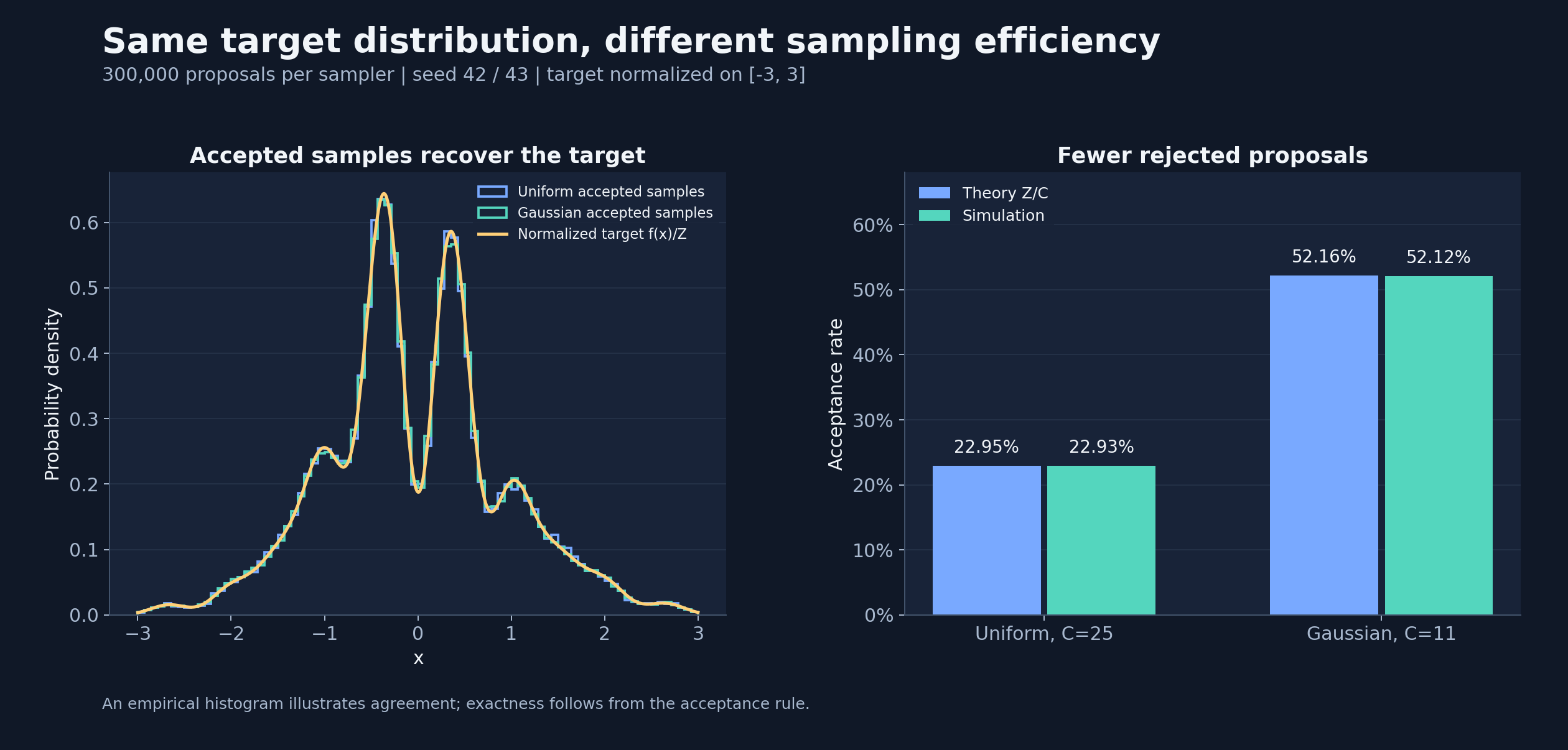
Figure 3. Both accepted-sample histograms track the same normalized target. The Gaussian proposal accepts a larger fraction of its candidates.

The observed rates are the simulation results shown in the supplied figures. Small differences in the target formula or its support change the normalizing constant and acceptance rate.

The histogram illustrates the result; the algebra explains why it works.

Part 4: Move from continuous curves to token probabilities

In vanilla speculative decoding, the proposal is the draft model’s categorical distribution over tokens. Use q for the draft and p for the target, both conditioned on the same prefix. [2]

A draft-token sampling step in PyTorch looks like this:

q = torch.softmax(draft_logits / temperature, dim=-1)
token = torch.multinomial(q, num_samples=1).item()

The token is drawn according to q. For example, probabilities [0.60, 0.30, 0.10] produce unequal token frequencies. A single draw using torch.multinomial is categorical sampling. [4]

The separate torch.rand draw is uniform. [5]

Draw	Distribution	Purpose
Draft token	Categorical distribution q	Propose the next token
Acceptance threshold	Uniform on [0, 1)	Decide whether to keep it
Correction token	Normalized positive difference of p and q	Replace a rejected proposal

For LLMs, sampling from the target is already straightforward once its logits are available. The expensive part is repeatedly computing those logits. Speculative decoding aims to amortize that computation across several candidate positions. [3]

Part 5: Speculative sampling changes the rejection procedure

Classical rejection sampling rejects a candidate and tries again. Speculative sampling uses a modified rule:

Accept a proposed token x with probability min(1, p(x) / q(x)).
On rejection, sample a replacement from normalized max(p − q, 0).

The acceptance and replacement steps belong together. We cannot simply remove the classical envelope constant and keep retrying from q. [2, 3]

Here is a vocabulary small enough to check by hand:

Token	Draft q	Target p	Acceptance probability
cat	0.60	0.30	0.50
dog	0.30	0.40	1.00
fox	0.10	0.30	1.00

The draft proposes too many cat tokens, so we keep half. We keep every dog and fox proposal.

Out of 10,000 proposals at this one fixed prefix, expected accepted counts are 3,000 cats, 3,000 dogs, and 1,000 foxes. That leaves 3,000 rejections to replace.

The missing probability mass is:

max(p − q, 0) = [0.00, 0.10, 0.20]

Normalize it to [0, 1/3, 2/3]. The replacements then contribute an expected 1,000 dogs and 2,000 foxes.

Final counts: 3,000 cats, 4,000 dogs, 3,000 foxes. We have recovered the target.

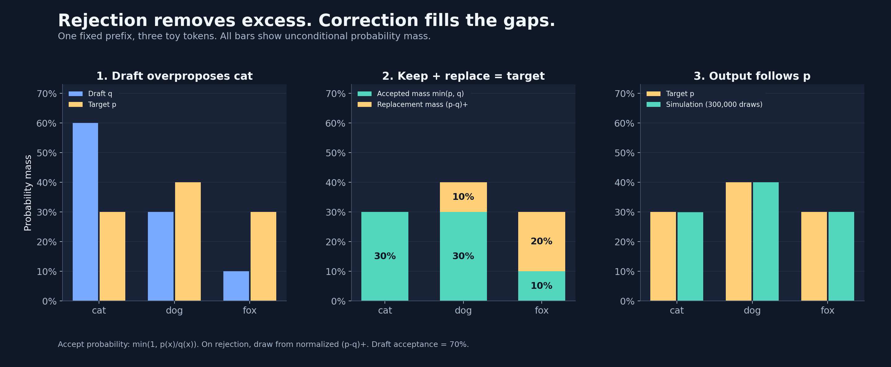
Figure 4. Teal accepted mass plus amber replacement mass equals the target. The simulation produces 29.926%, 40.032%, and 30.042%, close to the intended 30%, 40%, and 30%.

The bookkeeping fits in one identity:

$$\min(p(x),q(x))+\max(p(x)-q(x),0)=p(x).$$

Accepted drafts supply the first term. Rejections and their residual-distribution replacements supply the second term. Together they reproduce the target probabilities. The speculative-sampling papers establish this preservation property. [2, 3]

Part 6: Read the verification code with that picture in mind

Here is the core decision for one token position. Assume p and q are valid normalized vectors over the same vocabulary, and token was actually drawn from q.

# Probability of keeping this particular proposal.
acceptance = min(1.0, (p[token] / q[token]).item())

if torch.rand(1).item() < acceptance:
    output_token = token
else:
    # Weights for tokens underrepresented by accepted drafts.
    residual = (p - q).clamp_min(0)
    output_token = torch.multinomial(residual, 1).item()

torch.multinomial can use unnormalized, nonnegative weights with a positive sum, so explicit residual normalization is optional. [4]

A genuine rejection has positive residual mass in exact arithmetic. Production code also needs sound numerical handling; adding arbitrary probability floors changes the mathematical distribution.

If temperature, top-k, or top-p is used, the q in the ratio must match the distribution actually used to sample the draft. Likewise, p must represent the target decoding distribution we intend to preserve. [2, 3]

Part 7: Why verification stops at the first rejection

Imagine the draft proposes four tokens: A, B, C, D.

The target scores their positions in one causal forward pass using the proposed prefixes. If B is rejected and replaced, the scores for C and D were computed under a prefix we did not keep. We discard that suffix and start a new round.

If every proposal is accepted, the target distribution after the whole block supplies one bonus token. A round can therefore emit between one and gamma + 1 tokens. [2]

This also explains why output-token count and accepted-draft count need separate counters. A correction or bonus increases the output length without being an accepted draft.

Part 8: The engineering question: does drafting pay for itself?

Probability preservation establishes correctness. Speed depends on the costs.

At a fixed prefix, acceptance is the overlap between the distributions: alpha = sum(min(p, q)). A closer draft can increase that overlap, but its own computation may cost more. [2]

To make the tradeoff visible, consider a simple analytical model. Assume constant, independent acceptance probability alpha, target-pass cost of one unit, and draft-token cost c units:

$$\mathbb{E}[N]=\sum_{k=0}^{\gamma}\alpha^k,\qquad S(\alpha,\gamma,c)=\frac{\sum_{k=0}^{\gamma}\alpha^k}{1+c\gamma}.$$

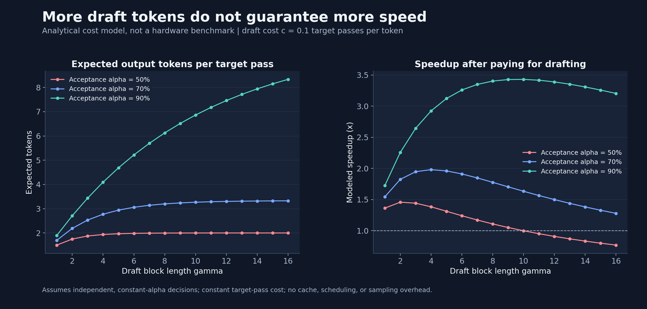
Figure 5. An analytical cost model with c = 0.1. These curves are not measured LLM benchmarks; target scoring cost and other overheads are idealized.

For alpha = 0.70, this model peaks near gamma = 4, at about 1.98×. Increasing the block further still produces more tokens per target call, but drafting costs grow faster than the remaining benefit. At alpha = 0.90, a longer block pays off.

This is a controlled calculation using the paper’s cost model, not a universal choice of gamma. [2]

One subtle point: a longer block does not inherently reduce each position’s acceptance probability. Even with constant alpha, the chance that the entire block survives is alpha^gamma. Later proposals are more likely to be discarded because an earlier proposal was rejected.

For a real implementation, I would measure end-to-end latency and output tokens per second, count accepted drafts separately, warm up both paths, and synchronize accelerator timing. KV-cache handling, vocabulary compatibility, batch size, and hardware all affect whether the theoretical opportunity becomes a speedup.

Part 9: What to Take Away

Classical rejection sampling provides the geometric intuition: a proposal supplies candidates, and a probability ratio filters them. Speculative sampling adds a residual correction so that every verification step produces a token with the target distribution.

The distinction matters in code. The categorical draw chooses a candidate; the uniform draw decides whether to keep it; the residual draw supplies probability mass that accepted drafts cannot provide. Together, those steps preserve the target distribution in exact arithmetic.

Whether that correctness translates into faster inference depends on draft cost, distribution overlap, and the serving implementation. The probability argument establishes what can be preserved. Measurement establishes what can be gained.

All five figures are embedded below their corresponding explanations. Select a chart to open the full-resolution image.

References

1. Kapil Sachdeva, What Is Rejection Sampling?, and the video introduction.
2. Yaniv Leviathan, Matan Kalman, and Yossi Matias, Fast Inference from Transformers via Speculative Decoding. See Algorithm 1 and sections 2–3.
3. Charlie Chen et al., Accelerating Large Language Model Decoding with Speculative Sampling. See section 4.2. This paper reverses the p/q naming convention; this post consistently uses p for target and q for draft.
4. PyTorch, torch.multinomial and Categorical.
5. PyTorch, torch.rand.