Medusa Part II: Candidate Trees, Verification, and Acceptance
August 31, 2026
A complete runtime guide to Medusa candidate pools, sparse rank trees, tree attention, greedy and typical acceptance, and an A100 trace.
Training a Medusa head only teaches it to propose future tokens. It does not make those proposals final output. At runtime, the original target model must still verify them.
This is the second of two articles. Part I: Architecture, Training, and Shifted Loss develops the heads and their loss. This article begins exactly where training ends.
Every inference iteration follows four decisions:
- The original LM head selects a root token.
- Every Medusa head supplies a top-K pool for its future position.
- A fixed sparse rank tree determines which combinations are worth verifying.
- Target-model logits and the selected acceptance rule determine which prefix is committed.
The distinction to keep throughout the article is:
Top-K selection decides what Medusa proposes. Greedy, rejection-sampling, or typical acceptance decides what the target allows into the output.
Part 1: One Medusa Inference Iteration, Without Skipping Steps
Consider a prompt ending with:
The cat
Assume the current final hidden state is . One forward pass produces:
Original LM head, top-1:  sat

Medusa head 0, top-2:    on, slept
Medusa head 1, top-2:    the, .
The original head predicts the root token sat. The two Medusa heads independently predict the next two positions after that root.
The complete candidates are:
sat on    the
sat on    .
sat slept the
sat slept .
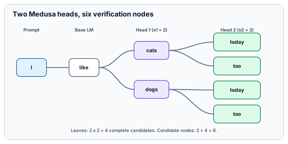
The implementation does not duplicate the prompt four times and run four ordinary target batches. It flattens the shared nodes into one tree and applies a special attention mask so each node sees only its own ancestors.
Suppose target verification says:
After "The cat"         target wants "sat"
After "The cat sat"     target wants "on"
After "The cat sat on"  target wants "the"
Then the path
sat on the
matches for its entire represented depth. One verification iteration commits three tokens:
root target token:       sat
accepted Medusa token 1: on
accepted Medusa token 2: the
The next iteration begins from the new prefix:
The cat sat on the
The selected verification node supplies the new final state and head logits. Those outputs produce new top-K lists, the same fixed tree topology is filled with new token IDs, and verification repeats.
If instead the target wanted slept after sat, the sat on ... paths would fail immediately. If one of the retained head-0 ranks contains slept, a path beginning with that rank can still win. If no retained rank matches, Medusa commits only sat and starts the next iteration.
This is the entire runtime loop:
prefill prompt
-> produce root and head distributions
-> fill candidate tree
-> verify tree with target backbone
-> choose longest accepted prefix
-> copy only selected KV-cache states
-> repeat from committed prefix
The draft heads do not recursively rerun while creating this tree. They generate their distributions from one backbone state. The target backbone is then run for tree verification. After the initial prompt prefill, that verification pass also supplies the selected base and Medusa logits needed to construct the next tree; there is no extra standalone prompt pass between decode iterations.
Part 2: Regular Tree Mathematics and the "250 Heads" Misreading
Let
The notation is one-based: refers to Python medusa_head[0].
For two levels with :
Depth 1 contains nodes.
Depth 2 contains nodes.
There are complete leaf continuations.
The number of additional non-root candidate nodes is
Including the root token from the original LM head:
For uniform Cartesian levels:
and
Therefore the expression
is exactly correct for a full five-level tree in which every parent at depth receives the same children.
Where an "Additional Length" near 250 comes from
The appendix of the Together AI launch post plots speed against Additional Length for different head configurations. Additional length counts flattened candidate-token positions, not learned heads.
The post does not provide the exact tuple for every plotted point, so consider this illustrative four-head configuration:
The depths contain
nodes, giving
This means:
- 4 Medusa heads participate.
- 150 complete leaf continuations exist.
- 255 non-root candidate-token nodes are verified.
- 256 total nodes exist if the LM-head root is included.
It does not mean that the model has approximately 250 prediction heads.
Why a full top-10 tree explodes
If four Medusa levels each retained ten children under every parent, then
With five levels it would become
Verifying that many nodes would destroy the latency benefit. This motivates a sparse, nonuniform tree.
Part 3: How Medusa Chooses an Optimized Sparse Tree
The optimized tree is chosen offline, not separately for every prompt.
Step 1: measure exact-rank accuracy
Run the trained Medusa heads on a calibration dataset. For head and rank , measure
This is an exact-rank statistic. If rank numbering begins at one,
The top-1 candidate may be correct frequently, rank 1 less frequently, and rank 9 only rarely. Farther heads also tend to be less accurate.
Step 2: score a rank path
A rank tuple such as
(0, 2, 1)
means:
- head 0 -> take its rank-0 token
- head 1 -> take its rank-2 token
- head 2 -> take its rank-1 token
Under the paper's independence approximation, the node score is
It estimates how often that rank combination will correctly extend the accepted prefix to that depth.
Step 3: grow a prefix-closed tree under a budget
Begin with the root. Repeatedly add the highest-scoring node whose parent is already present. Stop when the node budget is exhausted.
A toy calibration makes the behavior clear:
head 0: rank 0 = 0.60, rank 1 = 0.20 head 1: rank 0 = 0.50, rank 1 = 0.10
The candidate node scores include:
(0,) = 0.60 (1,) = 0.20 (0,0) = 0.60 x 0.50 = 0.30 (0,1) = 0.60 x 0.10 = 0.06 (1,0) = 0.20 x 0.50 = 0.10
The greedy order can begin:
(0,) -> (0,0) -> (1,) -> (1,0) -> (0,1)
The search goes deeper under a reliable top-ranked prefix before spending many nodes on unlikely branches. This produces the characteristic left-heavy tree.
For a prefix-closed tree , the paper approximates expected accepted length as
The optimization is therefore:
- maximize estimated accepted length,
- subject to a fixed node budget,
- and the rule that a node's parent must already exist.
The Medusa paper reports using AlpacaEval statistics to shape the sparse Vicuna-7B tree. It separately benchmarks tree sizes because a larger tree raises acceptance but also increases linear-layer and attention work. In its ablation, a sparse 64-node tree outperformed dense settings with 256 nodes. The optimum is a model-dataset-hardware property, not a universal constant.
A sparse tree needs depth counts, not one global
For a nonuniform tree, different parents retain different numbers of children. The number of nodes at depth is
where is the retained parent set and is the number of children assigned to parent .
Then
The Cartesian product formula is the special case in which every parent at the same depth has the same branching factor.
Part 4: The Real Vicuna-7B Reference Tree
The official loader selects the hard-coded vicuna_7b_stage2 topology for a Vicuna-7B model.
The checkpoint loader creates five trained Medusa heads. The candidate utility then computes
TOPK = 10
top_tokens = torch.topk(medusa_logits, TOPK, dim=-1).indices
so each head initially contributes a pool of ten ranked token IDs. Five heads produce pool entries.
TOPK=10 is only the candidate-pool width. It is not the number of children attached below every tree node.
The static tree contains rank tuples of maximum length four. Its depth counts are:
| Tree depth | Prediction source | Retained nodes | Distinct ranks used at that depth |
|---|---|---|---|
| 0 | Original LM-head root | 1 | top-1 root |
| 1 | Medusa head 0 | 10 | 0-9 |
| 2 | Medusa head 1 | 23 | 0-9, repeated below different parents |
| 3 | Medusa head 2 | 23 | 0-8, repeated below different parents |
| 4 | Medusa head 3 | 7 | 0-3, repeated below different parents |
| 5 | Medusa head 4 | 0 | unused by this topology |
Therefore
total nodes are evaluated, of which 63 are non-root choices.
At depth 2, the ten depth-1 parents receive different child counts:
depth-1 rank:       0  1  2  3  4  5  6  7  8  9
children retained: 10  5  2  2  1  1  1  1  0  0
Their sum is 23, not .
The sparse tree has 42 leaves:
 2 paths end at depth 1
14 paths end at depth 2
19 paths end at depth 3
 7 paths end at depth 4
------------------------
42 root-to-leaf paths
Those paths are padded to a common width of five positions:
1 root + at most 4 Medusa tokens = width 5
This explains the reference trace:
63 non-root choices
64 verified tree nodes
42 padded candidate paths
path width 5
Although the checkpoint carries five Medusa heads, this tree uses four future depths. The reference implementation still computes top-K values for all loaded heads before indexing the chosen tree; a tighter production kernel could skip a redundant head.
Part 5: Static Rank Topology, Dynamic Token Values
The tree file contains ranks, not vocabulary IDs and not words.
Suppose one inference iteration produces:
base LM root: "The"

head 0 ranks: 0=" cat", 1=" dog", 2=" model", ...
head 1 ranks: 0=" is",  1=" was", 2=" sat",   ...
head 2 ranks: 0=" a",   1=" on",  2=" very",  ...
The static tuple
(0, 2, 1)
is instantiated as
"The" + " cat" + " sat" + " on"
On the next iteration, (0, 2, 1) remains in the topology but maps to completely different token IDs because the head distributions changed.
This separates the two selection problems:
| Decision | When? | What decides it? |
|---|---|---|
| Which rank tuples deserve tree nodes? | Offline | Calibration accuracies plus a node budget |
| Which actual token occupies each tuple position? | Every inference iteration | Current head top-K logits |
| Which candidate prefix is committed? | Every verification iteration | Current target-model logits |
The offline score never overrides the target model at runtime. It only decides which proposals are worth presenting to the target.
Part 6: Tree Attention Verifies Shared Prefixes Once
If we expanded every leaf into a separate batch row, shared prefixes would be duplicated. Tree attention represents each distinct node once.
For the official Vicuna tree, the principal tensors are conceptually:
tree_candidates:      [1, 64]
tree attention mask:  [1, 1, 64, 64]
tree position IDs:    [64]
retrieved paths:      [42, 5]
verifier logits:      [42, 5, vocabulary]
The exact dimensions can acquire singleton axes inside the implementation, but the semantics are stable.
The attention mask grants a node access to:
- every original prompt token,
- the root candidate,
- only the candidate nodes on its own ancestor path.
It cannot attend to siblings or tokens from another continuation. Position IDs are assigned by tree depth, so two siblings occupy the same logical sequence position even though they have different flattened indices.
After the target forward pass, retrieval indices reconstruct 42 padded root-to-leaf paths from the 64 node outputs. Only KV-cache entries belonging to the selected accepted path are copied into the contiguous decode cache. The other verified branches are discarded.
This is why production Medusa is neither:
four prompts copied into a normal batch
nor:
four separate target-model forward passes.
It is one tree-shaped target pass with shared prefix nodes and a custom causal mask.
Part 7: Exact Greedy Verification and Rejection
Let
candidates.shape       = [number_of_paths, path_width]
verifier_logits.shape  = [number_of_paths, path_width, vocabulary]
candidates[:, 0] is the root token already selected by the ordinary LM head. For every later position, the target logit at the previous position predicts the candidate token:
target_tokens = verifier_logits[:, :-1].argmax(dim=-1)
matches = candidates[:, 1:] == target_tokens
prefix_matches = matches.int().cumprod(dim=1)
accepted_per_path = prefix_matches.sum(dim=1)
cumprod enforces the left-to-right rule:
raw matches:     [True, False, True, True]
valid prefix:    [1,    0,     0,    0]
accepted length: 1
The later True values do not count after an earlier rejection.
The reference implementation chooses
accept_length = accepted_per_path.max()
best_candidate = accepted_per_path.argmax()
and appends
candidates[best_candidate, :accept_length + 1]
The +1 includes the root token.
Define the metrics carefully:
Therefore:
| Verification outcome | Accepted Medusa tokens | Committed tokens |
|---|---|---|
| Every proposal fails immediately | 0 | 1 root |
| One future token matches | 1 | 2 |
| Four future tokens match | 4 | 5 |
If all paths accept zero Medusa tokens, the implementation selects path 0 by convention. The choice is harmless because every path shares the same root and only that root is committed.
If several paths tie at a positive greedy prefix length, their accepted token prefix must agree with the same target argmax sequence. Their unaccepted suffixes may differ; choosing the first maximum does not change the committed text.
Padded paths are not real completions
The 42 leaves have different depths but are stored at width five. Short paths use a sentinel retrieval index that maps to token ID 0 in the reference code. With the Vicuna tokenizer, ID 0 decodes as <unk>.
Consequently, a diagnostic trace may say that Medusa proposed <unk> immediately after an accepted prefix. Sometimes that is not a genuine head proposal--it means the selected leaf ended and the next tensor slot was padding. A correct trace should distinguish
first real candidate mismatch
from
selected path exhausted
rather than interpreting every padded ID as a proposal.
Part 8: What Is Actually Guaranteed?
The phrase "Medusa is lossless" needs an acceptance rule attached to it.
Before comparing the rules, separate two operations that are easy to mix up:
Medusa-head top-K       decides which tokens enter the candidate tree
target acceptance rule  decides which candidate prefix becomes output
Every Medusa head produces a distribution over the complete vocabulary. The reference implementation extracts a top-10 pool from each head, then the sparse topology chooses particular rank combinations from those pools. This happens before acceptance. Taking top-K candidates does not imply that typical acceptance is being used.
Greedy exact verification
When every accepted Medusa token must equal the target model's greedy argmax, the committed sequence matches ordinary greedy decoding from that same target. Medusa can change the number of tokens committed per step, not their values.
Greedy decoding does not sample. For example, suppose the target distribution at one verified position is:
the:   0.35
a:     0.25
its:   0.18
that:  0.12
this:  0.10
The target token is deterministically the:
target_token = probabilities.argmax()  # "the"
accepted = medusa_candidate == target_token
A Medusa proposal of a is rejected in greedy mode even though the target assigns it probability .
There is still no guarantee that a speculative token is accepted. The guarantee is:
at least one target root token is committed per iteration
not:
every Medusa head contributes one accepted token
Distribution-preserving rejection sampling
For stochastic decoding, a proper speculative rejection-sampling correction can preserve the target distribution. This uses the draft and target probabilities, not a simple equality test.
Typical acceptance
For nonzero-temperature decoding, the original Medusa paper also proposes an optional typical-acceptance rule. Instead of requiring the target's top-1 token, it asks whether the proposed token is sufficiently plausible under the target distribution:
Here is a fixed ceiling and adapts to the target's uncertainty. Higher entropy makes smaller, lowering the threshold and allowing more plausible alternatives. The reference generation entry point uses
The implementation computes from temperature-scaled verifier logits:
target_probabilities = softmax(verifier_logits / temperature)
threshold = min(
    posterior_threshold,              # paper epsilon
    exp(-entropy) * posterior_alpha,  # paper delta * exp(-H)
)
Changing the temperature therefore changes both the candidate probabilities and their entropy-dependent threshold.
For the five-token distribution above, the entropy is approximately
so the threshold is
The result is:
| Proposed token | Target probability | Greedy exact | Typical threshold test |
|---|---|---|---|
the |
0.35 | Accept | Accept |
a |
0.25 | Reject | Accept |
its |
0.18 | Reject | Accept |
that |
0.12 | Reject | Accept |
this |
0.10 | Reject | Accept |
This table does not mean that Medusa randomly chooses one of the five tokens. It means that if any of them already appears in a candidate-tree path, it passes the typical test at this position.
A complete typical-acceptance path
Return to the prompt:
The cat
Suppose the original LM head selects the root sat, while one tree path assembled from the Medusa-head top-K pools is
sat -> on -> a -> mat
The root sat is committed first. The target then verifies the three Medusa proposals under their correct conditional prefixes:
| Medusa proposal | Target probability | Entropy | Threshold | Result |
|---|---|---|---|---|
on after The cat sat |
0.50 | 1.33 | 0.079 | Accept |
a after The cat sat on |
0.25 | 1.51 | 0.066 | Accept |
mat after The cat sat on a |
0.05 | 1.43 | 0.072 | Reject |
Acceptance must form one consecutive prefix, so verification stops at mat. This iteration commits
sat on a
That is one root token plus two accepted Medusa tokens.
Is typical acceptance deterministic?
The threshold itself is a deterministic membership test:
acceptable = target_probability_of_candidate > threshold
In the official fast path, all existing tree candidates are tested this way. Medusa selects the path with the longest accepted prefix; if equal-length paths tie, it selects the one with the greatest cumulative target log-likelihood. Given the same logits and tree, this path is deterministic.
A separate sampling variant can remove tokens below the threshold, renormalize the remaining probabilities, and sample one of them. That version is stochastic. Therefore, "typical acceptance" should not automatically be read as "randomly select any token above the threshold."
The first root token is still selected greedily in the official fast path. Typical acceptance can admit more Medusa tokens at nonzero temperature, but it deliberately relaxes exact target-distribution matching. "Similar generation quality" is not the same claim as "identical target distribution."
In every mode, the idea that Medusa has "no target" is incorrect. The same LLM that supplied the hidden state also acts as the verifier during the tree pass.
Part 9: Running a Real Pretrained Medusa Checkpoint
The repository includes an instrumented inference runner for the official FasterDecoding/medusa-vicuna-7b-v1.3 checkpoint:
Colab/A100 requirements
In a fresh Colab A100 runtime, clone this repository and install the pinned compatibility set:
python -m pip install -r examples/requirements-medusa-pretrained.txt
The requirements file installs the official Medusa repository together with its intentionally conservative Transformers stack. If your runtime already includes a CUDA-enabled PyTorch build, keep that GPU build rather than replacing it with a CPU wheel.
Keep Colab's CUDA-enabled PyTorch rather than pinning a second Torch wheel. Then run:
python examples/medusa_pretrained_trace.py \
    --prompt "Explain why speculative decoding is lossless." \
    --max-new-tokens 96 \
    --dtype float16 \
    --output-json medusa_trace.json
The script directly calls the official primitives:
initialize_medusagenerate_candidatestree_decodingevaluate_posteriorupdate_inference_inputs
It independently reconstructs the greedy prefix mask and asserts that its accepted length agrees with the official utility.
Why the loader says the heads were newly initialized
The checkpoint is loaded in three steps:
- Load the Vicuna base model.
- Construct Medusa-head modules.
- Load
medusa_lm_head.ptinto those modules.
Transformers prints its "newly initialized" warning during step 1, before the separate head file is applied. In the official loading path, that warning is expected and does not by itself mean the final heads remain random.
The old uploaded configuration also reports too few heads. The official loader contains a compatibility workaround that constructs five heads before loading the separate state dictionary. This is why using AutoModel directly is not equivalent to using MedusaModel.from_pretrained(...).
These other startup messages are also informational:
_register_pytree_nodeis a compatibility deprecation warning from the older Transformers version.- "legacy" Llama tokenization preserves the tokenizer behavior expected by Vicuna.
- The first run downloads the Vicuna base shards and the separate Medusa weights; later runs use the Hugging Face cache.
What one A100 trace showed
One run used a 50-token prompt and generated at least 96 new tokens. Representative iterations were:
| Iteration | Match mask after root | Accepted Medusa tokens | Total committed | Committed text fragment |
|---|---|---|---|---|
| 1 | [False] |
0 | 1 | Spe |
| 2 | [True, False] |
1 | 2 | culative |
| 3 | [True, True, True, True] |
4 | 5 | decoding is a technique |
| 18 | [True, True, True, False] |
3 | 4 | current frame. This |
Iteration 1 illustrates the zero-acceptance case:
root token from base LM:  "Spe" -> committed
head-0 candidate:         "spe"
target continuation:      "cul" -> mismatch
Iteration 3 illustrates a full-depth match. The target accepted four Medusa tokens after the root, so one verification committed five tokens.
Across all 45 iterations:
accepted Medusa tokens:              52
total committed tokens:              97
mean accepted Medusa / iteration:   1.156
mean committed / iteration:         2.156
The acceptance-length distribution was:
| Accepted Medusa tokens | Number of iterations |
|---|---|
| 0 | 9 |
| 1 | 23 |
| 2 | 11 |
| 3 | 1 |
| 4 | 1 |
The first tree iteration took about 148 ms because it included warm-up effects. The remaining 44 iterations averaged approximately 40.47 ms with a median near 40.12 ms on that runtime.
Tokens per verification step are not wall-time speedup
The ratio
is a decode-step compression ratio. It says how much sequence progress the average tree pass made.
It is not automatically a latency speedup. A 64-node tree pass is more expensive than a one-token decode pass. Wall-time speedup requires an ordinary greedy baseline with the same:
- target model,
- prompt set and output lengths,
- dtype and quantization,
- GPU,
- sampling configuration,
- warm-up procedure,
- cache implementation.
A useful approximation is
but the final number should be measured rather than inferred.
What should be verified against a baseline?
For greedy exact mode, compare the complete generated token-ID sequence against ordinary greedy generation from the base target. Text comparison alone can hide tokenizer cleanup differences.
The repository also contains a small educational implementation that trains Medusa-1 heads and performs this exact baseline-ID comparison:
Small Medusa-1 training and verification demo
Install its small dependency set from the demo requirements file. That teaching script expands candidate leaves into a normal batch so every probability and rejection is easy to inspect. It is not a production speed benchmark. The pretrained runner uses the official flattened tree, custom position IDs, tree mask, and KV-cache update.
Part 10: Production Measurements That Matter
Head loss is useful, but it does not establish inference speed. A complete evaluation should include:
| Metric | Why it matters |
|---|---|
| Per-head cross-entropy | Shows how uncertainty grows with prediction distance |
| Exact-rank and top-K accuracy | Supplies statistics for sparse-tree design |
| Accepted Medusa tokens per iteration | Measures useful speculative depth |
| Committed tokens per iteration | Includes guaranteed root progress |
| Acceptance-length histogram | Reveals whether averages hide frequent zero-accept steps |
| Tree node count and leaf count | Quantifies verification breadth and path coverage |
| Ordinary decode latency | Establishes the real denominator for speedup |
| Tree verification latency | Measures added compute from speculative nodes |
| Target calls per generated token | Measures reduction in sequential target work |
| Time to first token | Usually dominated by prefill rather than Medusa drafting |
| Inter-token latency | Captures the main low-batch user-visible benefit |
| Throughput under concurrency | Shows whether normal batching already saturates compute |
| Peak memory and KV-cache memory | Captures head, buffer, and serving overhead |
| Exact baseline token-ID match | Validates greedy losslessness |
Tree selection should be calibrated on output resembling production traffic. A code-tuned tree may waste nodes on chat, and a chat-tuned tree may underperform on structured generation. The optimum can also move between an A100, H100, and a highly concurrent server because the cost of verifying additional nodes changes.
The right optimization target is not maximum acceptance in isolation. It is approximately
Adding a low-probability node can raise expected acceptance slightly while making every iteration slower. That is why the Medusa paper observed diminishing and eventually negative returns as trees grew.
Common Inference Misreadings
| Misreading | Correct interpretation |
|---|---|
| "Top-K candidate generation is typical acceptance." | Top-K creates the proposal pool. Acceptance is a later target-verification decision. |
| "Greedy decoding samples the highest-probability token." | Greedy decoding does not sample; it deterministically takes the argmax. |
| "Typical acceptance randomly chooses any token above the threshold." | The official fast path tests existing tree candidates, selects the longest valid prefix, and uses likelihood to break equal-length ties. A sampling variant can be stochastic. |
| "Additional length 250 means 250 heads." | It counts flattened candidate-token nodes; a few heads can create hundreds of nodes. |
| "Top-K is 10, so every node has ten children." | Ten is the per-head candidate-pool width; the sparse topology retains only selected rank combinations. |
| "The tree contains 63 total tokens." | The reference configuration contains 63 non-root choices plus one LM-head root, for 64 verification nodes. |
| "There are 64 candidate completions." | There are 64 nodes but 42 root-to-leaf paths in the Vicuna-7B configuration. |
| "Because the heads belong to the LLM, their output is automatically accepted." | The original target backbone verifies the tree and can reject every speculative token. |
| "At least one Medusa token is guaranteed." | Only the root target token is guaranteed; accepted Medusa tokens may be zero. |
| "Typical acceptance is exactly lossless." | Exact greedy matching or proper rejection sampling can preserve target behavior. Typical acceptance deliberately relaxes exact distribution equality. |
| "2.156 committed tokens per iteration means 2.156x speedup." | It measures sequence progress per verification call; wall speed also depends on tree-pass latency. |
Part II Summary
- Each head produces a full vocabulary distribution; top-K extracts a candidate pool.
- A regular Cartesian tree quickly becomes too large, so Medusa uses an offline-optimized sparse rank topology.
- Runtime top-K token IDs fill that fixed topology with prompt-dependent values.
- Tree attention verifies shared nodes once while preserving the causal ancestry of every path.
- Greedy verification accepts only consecutive tokens equal to the target argmax.
- Typical acceptance instead allows target-plausible proposals above an entropy-adaptive threshold.
- The official fast typical path is a deterministic validation rule; stochastic typical sampling is a separate variant.
- One root token is always committed, but zero Medusa tokens may be accepted.
- Committed tokens equal one root plus the accepted Medusa prefix.
- Acceptance length measures step compression, not wall-clock speedup by itself.
The complete mental model is:
The heads create possibilities. Top-K forms candidate pools. The sparse tree selects combinations worth checking. Tree attention checks them together. The target model and acceptance rule decide which prefix becomes output.
Return to Part I: Architecture, Training, and Shifted Loss for the training path.