Medusa Part I: Architecture, Training, and Shifted Loss
August 31, 2026
A tensor-level guide to Medusa heads, frozen and joint training, label shifts, and the complete shifted cross-entropy calculation.
Autoregressive language models have an awkward hardware problem: a decoding step moves billions of parameters through the GPU and usually produces only one token. Speculative decoding improves that ratio by letting a cheap draft model propose several tokens and asking the expensive target model to verify them together. It works, but now the serving system owns two models.
Medusa asks a beautifully direct question:
What if the target model carried its own lightweight drafting mechanism?
It adds several future-token prediction heads to one LLM, turns their top predictions into a candidate tree, verifies that tree with the same LLM, and commits the longest accepted prefix. There is no separately hosted draft model.
That one-sentence description hides most of the details that matter in an implementation:
- Does every head receive the same hidden state?
- Which token is head 0 trained to predict?
- Is the target model frozen?
- Is the candidate tree used during training?
- How is each auxiliary loss shifted against the labels?
This first article follows the training path in chronological order: what the heads consume, which future token each head predicts, which parameters change in Medusa-1 and Medusa-2, and how shifted cross-entropy aligns every head with its labels. Part II begins exactly where training ends.
The central mental model is:
Medusa has one target LLM, lightweight auxiliary draft heads, and a target-verification pass. The draft heads propose; the original LM decides.
A Short Historical Map
The terminology became confusing because related ideas arrived with different training and architectural choices.
| Year | Work | Important change |
|---|---|---|
| 2018 | Blockwise Parallel Decoding | Used multiple output heads to predict future positions in parallel. |
| 2023 | Together AI's Medusa post | Introduced Medusa heads, tree attention, typical acceptance, and the head-configuration ablation. |
| 2024 | Medusa technical report | Formalized Medusa-1, Medusa-2, self-distillation, and optimized sparse trees. |
| 2024 | Better & Faster LLMs via MTP | Made parallel future-token prediction a pretraining objective with independent heads. |
| 2024-2025 | DeepSeek-V3 | Used sequential MTP modules that preserve a causal chain between future positions. |
| 2025 onward | FastMTP and vLLM Speculators MTP | Reused a native MTP prediction layer recursively and fine-tuned it for speculation. |
All of these methods predict multiple future tokens. They are not all the same network.
Part 1: Why Decoding One Token at a Time Is Expensive
Let the current tokenized context be
The Transformer backbone produces a final hidden state at the last position:
The ordinary language-model head maps it to one score per vocabulary token:
where is the hidden width and is the vocabulary size. Greedy decoding chooses
The new token is appended, and another decoding step is needed for . The dependency is sequential:
At low batch sizes, decoding is commonly memory-bandwidth-bound: the GPU repeatedly reads the large model weights while doing too little arithmetic per read. The objective is not to make the target model cheaper. It is to obtain several useful tokens from one expensive target-model interaction.
Keep the tensor names distinct:
- is a hidden vector of length .
- is a logit vector of length .
argmax(logits)is a token ID.- Decoding that token ID produces a text fragment, which may be only part of a word.
This distinction becomes important when several heads all consume the same hidden state but emit different vocabulary distributions.
Part 2: Vanilla Speculative Decoding Still Has a Target
Traditional speculative decoding introduces two autoregressive models:
- A cheap draft model proposes tokens.
- The expensive target model evaluates those proposed positions in one forward pass.
For greedy generation, verification is easy to state. Starting at the first drafted position, accept tokens while
The first mismatch ends the accepted prefix. A later token cannot be accepted after an earlier rejection because its context contains the rejected token.
For sampling, exact speculative decoding uses a rejection-sampling correction involving both and . That procedure can preserve the target distribution exactly. The mathematical details are covered in Unpacking Speculative Decoding.
Two guarantees are often mixed together:
- Progress: every iteration can commit at least one target-approved token.
- Draft acceptance: there is no guarantee that even one speculative token will be accepted.
If every draft token is wrong, generation still advances by one target token. Speculation changes how many target-approved tokens can be harvested from a verification step; it never removes the verifier.
The operational cost is that the draft model brings its own parameters, KV cache, checkpoint lifecycle, device placement, and distributed-serving configuration. Medusa removes that separately hosted model--not the verification step.
Part 3: Medusa Puts the Draft Heads on the Target Model
Assume we attach Medusa heads. At position , the prediction roles are
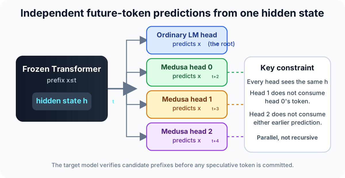
There is still only one Transformer backbone. The four prediction modules receive the same final backbone representation.
This gives us three precise statements:
medusa_num_heads = 3means three additional heads plus the original LM head.- Head 1 does not consume the token selected by head 0.
- A later Medusa head does not receive more observed context than an earlier one.
Each head models a different marginal distribution from the same prefix:
The heads are parallel and conditionally independent given in the architecture. The future tokens themselves are not independent in natural language; that mismatch is why farther heads are harder to train.
What is inside one Medusa head?
The Medusa report uses a residual feed-forward transformation followed by a vocabulary projection:
The shapes are
A compact PyTorch version is:
class ResidualBlock(nn.Module):
    def __init__(self, hidden_size):
        super().__init__()
        self.linear = nn.Linear(hidden_size, hidden_size)
        nn.init.zeros_(self.linear.weight)
        nn.init.zeros_(self.linear.bias)

    def forward(self, hidden_states):
        return hidden_states + F.silu(self.linear(hidden_states))

class MedusaHead(nn.Module):
    def __init__(self, hidden_size, vocab_size, lm_head_weight):
        super().__init__()
        self.residual = ResidualBlock(hidden_size)
        self.vocab_projection = nn.Linear(
            hidden_size,
            vocab_size,
            bias=False,
        )

        with torch.no_grad():
            self.vocab_projection.weight.copy_(lm_head_weight)

    def forward(self, hidden_states):
        return self.vocab_projection(self.residual(hidden_states))
The residual block starts as the identity because its learned branch is zero-initialized. The vocabulary projection is initialized from the original LM head, but every Medusa head owns and subsequently trains its own copy.
Three heads therefore mean three residual blocks and three vocabulary projections--not one projection evaluated at three offsets.
Part 4: Medusa-1 and Medusa-2 Train Different Parameter Sets
The candidate tree does not exist during head training. Training first teaches future-token distributions; inference later turns those distributions into a tree.
Medusa-1: freeze the complete target model
Medusa-1 starts from an already trained LLM and freezes:
- token embeddings,
- all Transformer layers,
- normalization layers,
- the original language-model head.
Only the new Medusa heads are trainable:
for parameter in base_model.parameters():
    parameter.requires_grad_(False)

medusa_heads = nn.ModuleList(
    MedusaHead(
        hidden_size=base_model.config.hidden_size,
        vocab_size=base_model.config.vocab_size,
        lm_head_weight=base_model.get_output_embeddings().weight,
    )
    for _ in range(number_of_medusa_heads)
)

optimizer = torch.optim.AdamW(
    medusa_heads.parameters(),
    lr=1e-3,
)
The frozen model still runs a forward pass to produce . Frozen means that its parameters receive no optimizer update; it does not mean the backbone is absent from training.
Because the original model weights do not change, its ordinary next-token behavior remains intact. This makes Medusa-1 a post-hoc, parameter-efficient augmentation.
Medusa-2: update the target and the heads jointly
Medusa-2 jointly trains the target backbone and Medusa heads. The report uses a combined objective, differential learning rates, and head warm-up so the large auxiliary gradients do not damage next-token capability.
| Property | Medusa-1 | Medusa-2 |
|---|---|---|
| Starting point | Existing target LLM | Existing or jointly fine-tuned LLM |
| Backbone | Frozen | Trainable |
| Token embeddings | Frozen | May be updated with backbone recipe |
| Original LM head | Frozen | Protected by ordinary LM loss |
| Auxiliary heads | Trained | Trained |
| Main reason to use it | Cheap, post-hoc augmentation | Better head accuracy and acceptance |
| Original checkpoint behavior preserved | Yes, because target weights are unchanged | Not byte-for-byte; the jointly trained model becomes the new target |
The report measured about wall-time speedup for Medusa-1 and for Medusa-2 in its Vicuna-7B case study. These are workload- and implementation-specific measurements, not universal multipliers.
Part 5: The Loss Is Shifted Cross-Entropy
Suppose a token sequence is
The logit-to-label alignment is:
| Prediction source | logits[:, t] predicts |
Shift |
|---|---|---|
| Original LM head | labels[:, t + 1] |
1 |
| Medusa head 0 | labels[:, t + 2] |
2 |
| Medusa head 1 | labels[:, t + 3] |
3 |
| Medusa head 2 | labels[:, t + 4] |
4 |
For zero-based Python head index ,
The reusable function is:
def shifted_cross_entropy(
    logits,
    labels,
    shift,
    ignore_index=-100,
):
    """logits[:, t] predicts labels[:, t + shift]."""
    if shift <= 0:
        raise ValueError("shift must be positive")
    if logits.size(1) <= shift:
        raise ValueError("sequence is too short for this head")

    shifted_logits = logits[:, :-shift, :].contiguous()
    shifted_labels = labels[:, shift:].contiguous()

    return F.cross_entropy(
        shifted_logits.reshape(-1, shifted_logits.size(-1)).float(),
        shifted_labels.reshape(-1),
        ignore_index=ignore_index,
    )
For sequence length :
| Predictor | Logit positions | Label positions | Valid pairs |
|---|---|---|---|
| Base, shift 1 | 4 | ||
| Medusa 0, shift 2 | 3 | ||
| Medusa 1, shift 3 | 2 | ||
| Medusa 2, shift 4 | 1 |
Farther heads lose more training positions at the right sequence boundary. With packed long sequences this is a small fraction; with toy sequences it is impossible to ignore.
Full calculation: batch 2, sequence length 3, vocabulary 5
Use this vocabulary:
0=<pad>, 1=I, 2=like, 3=cats, 4=dogs
Our batch is
with shape
[batch, sequence] = [2, 3].
Every Medusa head emits logits of shape
[batch, sequence, vocabulary] = [2, 3, 5].
For Medusa head 0, shift=2:
shifted_logits = logits[:, :-2, :]  # [2, 1, 5]
shifted_labels = labels[:, 2:]      # [2, 1]
Only position is valid in each example:
Example 0: logits[0, 0] predicts labels[0, 2] = cats Example 1: logits[1, 0] predicts labels[1, 2] = dogs
Assume the two relevant logit vectors are
For example A, the probability of the target cats is
Its negative log-likelihood is
For example B:
and
PyTorch's default cross-entropy reduction averages the two valid batch-position pairs:
Nothing is calculated for logits[:, 1] or logits[:, 2] for this head because the corresponding labels would lie beyond the sequence.
Medusa head 1 would require shift=3. With ,
logits[:, :-3, :]  # empty
labels[:, 3:]      # empty
so that head cannot be trained from this toy block. A robust implementation must skip it or reject the batch rather than pass empty tensors into cross-entropy.
Combining multiple head losses
Medusa-1 downweights more distant heads:
def medusa1_loss(medusa_logits, labels, decay=0.8):
    per_head = []

    for head_index, logits in enumerate(medusa_logits):
        loss = shifted_cross_entropy(
            logits,
            labels,
            shift=head_index + 2,
        )
        per_head.append(loss)

    total = sum(
        decay ** (index + 1) * loss
        for index, loss in enumerate(per_head)
    )
    return total, per_head
Medusa-2 also protects next-token prediction with the ordinary LM loss:
The original next-token loss is unnecessary for updating a frozen Medusa-1 backbone, although it can still be logged as a baseline metric.
Why the later-head loss is usually higher
The later head does not have more context. All independent Medusa heads see , which represents only .
Head 0 models without seeing . Head 2 models without seeing . Conditional uncertainty generally grows with distance, so the aggregate tendency is
That is a dataset-level tendency, not a guarantee for every batch. Boundary effects also give farther heads fewer valid examples.
At this point training is complete. There has been no top-K selection, no candidate tree, and no rejection. Those are inference operations.
Part I Summary
- One target LLM supplies the shared hidden state and the ordinary next-token head.
- Medusa adds independent residual heads for progressively farther future positions.
- Python Medusa head 0 predicts two positions ahead, so head uses label shift .
- Medusa-1 freezes the target and trains only the auxiliary heads.
- Medusa-2 jointly updates the target and heads while retaining the ordinary LM objective.
- The candidate tree, top-K pools, verification, and rejection belong to inference, not head training.
Continue with Part II: Candidate Trees, Verification, and Acceptance.
References
- Stern et al., Blockwise Parallel Decoding for Deep Autoregressive Models
- Together AI, Medusa: Simple Framework for Accelerating LLM Generation with Multiple Decoding Heads
- Cai et al., Medusa: Simple LLM Inference Acceleration Framework with Multiple Decoding Heads
- FasterDecoding, official Medusa implementation
- Gloeckle et al., Better & Faster Large Language Models via Multi-token Prediction
- DeepSeek-AI, DeepSeek-V3 Technical Report
- Cui et al., FastMTP: Accelerating LLM Inference with Enhanced Multi-Token Prediction